GRIM in depth

This vignette builds on vignette("grim"), which covers the basics of GRIM testing with grim() and grim_map(). Here are the numbers behind a test result, the settings recorded with it, the values around the reported ones with grim_map_seq() and grim_map_total_n(), and the GRIM statistics behind the exp_incon column.

Behind a test result

Reconstructed values

With show_rec = TRUE, the output includes the numbers on which the test result is based:

pigs1 |>
  grim_map(digits_x = 2, items_averaged = 1, data_type = "integer", show_rec = TRUE) |>
  dplyr::select(x, n, consistency, rec_sum:rec_x_lower)
#> # A tibble: 12 × 8
#> # GRIM: show_rec = TRUE
#>        x     n consistency rec_sum sum_lower sum_upper rec_x_upper rec_x_lower
#>    <dbl> <int> <lgl>         <dbl>     <dbl>     <dbl>       <dbl>       <dbl>
#>  1  7.22    32 TRUE         231.0        231       231       7.25       7.219 
#>  2  4.74    25 FALSE        118.5        119       118       4.76       4.72  
#>  3  5.23    29 FALSE        151.7        152       151       5.241      5.207 
#>  4  2.57    24 FALSE         61.68        62        61       2.583      2.542 
#>  5  6.77    27 FALSE        182.8        183       182       6.778      6.741 
#>  6  2.68    28 TRUE          75.04        75        75       2.714      2.679 
#>  7  7.01    29 FALSE        203.3        204       203       7.034      7     
#>  8  7.38    26 TRUE         191.9        192       192       7.385      7.346 
#>  9  3.14    27 FALSE         84.78        85        84       3.148      3.111 
#> 10  6.89    31 FALSE        213.6        214       213       6.903      6.871 
#> 11  5       25 TRUE         125          125       125       5          5     
#> 12  0.24    28 FALSE          6.72         7         6       0.25       0.2143

• rec_sum is x * n * items_averaged, the sum implied by the reported mean. The sum of integer data is a whole number, which rec_sum generally is not.
• sum_lower and sum_upper are the smallest and largest whole-number sums that would have been reported as x. A value set is consistent if and only if sum_lower <= sum_upper. If it is inconsistent, they are the whole numbers just above and below rec_sum, so their difference is always 1 and says nothing about how far off the mean is.
• rec_x_upper and rec_x_lower are the two achievable means closest to x: rec_sum rounded up and down, divided by n * items_averaged. They show how far the reported mean is from an achievable one. With x_meaning = "percentage", they are percentages like x.

Recorded settings

A mapper records the settings of its call on its output, so that a report can state the conditions of each result. scrutiny_meta() returns them:

pigs1 |>
  grim_map(digits_x = 2, items_averaged = 1, data_type = "integer", rounding = "up") |>
  scrutiny_meta()
#> # A tibble: 5 × 4
#>   setting   value  default added_by
#>   <chr>     <chr>  <lgl>   <chr>   
#> 1 x_meaning 'mean' TRUE    grim_map
#> 2 rounding  'up'   FALSE   grim_map
#> 3 threshold 5      TRUE    grim_map
#> 4 symmetric FALSE  TRUE    grim_map
#> 5 show_rec  FALSE  TRUE    grim_map

default says whether a setting was left at its default. explain_map() and grim_plot_grid() read the settings from there, so they apply the same rounding method as the call. For the same reason, dplyr::bind_rows() refuses to combine the output of calls with different settings, whose rows would otherwise be read under the first call’s settings.

Achievable means

grim_values() returns all means that a sample of n integers can have and that would be reported as x, each with the whole-number sum behind it:

grim_values(x = 5.19, n = 32, digits_x = 2, items_averaged = 1, data_type = "integer")
#> # A tibble: 1 × 5
#>    case     x     n items_averaged   sum
#>   <int> <dbl> <int>          <int> <dbl>
#> 1     1 5.188    32              1   166
grim_values(x = 5.19, n = 300, digits_x = 2, items_averaged = 1, data_type = "integer")
#> # A tibble: 3 × 5
#>    case     x     n items_averaged   sum
#>   <int> <dbl> <int>          <int> <dbl>
#> 1     1 5.187   300              1  1556
#> 2     1 5.19    300              1  1557
#> 3     1 5.193   300              1  1558
grim_values(x = 5.19, n = 28, digits_x = 2, items_averaged = 1, data_type = "integer") # inconsistent: none
#> # A tibble: 0 × 5
#> # ℹ 5 variables: case <int>, x <dbl>, n <int>, items_averaged <int>, sum <dbl>

grim_closest() returns the achievable mean nearest to x, with the sum behind it, in one row per value set. If x is consistent, that is the nearest one that would be reported as x:

grim_closest(x = 5.19, n = 28, digits_x = 2, items_averaged = 1, data_type = "integer")
#> # A tibble: 1 × 5
#>    case     x     n items_averaged   sum
#>   <int> <dbl> <int>          <int> <dbl>
#> 1     1 5.179    28              1   145

Both functions are vectorized. A reported mean may have one achievable mean, several, or none, so grim_values() returns one row per achievable mean, and case says which value set it belongs to. An inconsistent value set has no rows:

grim_values(
  x = c(5.19, 5.19, 5.19),
  n = c(32, 300, 28),
  digits_x = 2,
  items_averaged = 1,
  data_type = "integer"
)
#> # A tibble: 4 × 5
#>    case     x     n items_averaged   sum
#>   <int> <dbl> <int>          <int> <dbl>
#> 1     1 5.188    32              1   166
#> 2     2 5.187   300              1  1556
#> 3     2 5.19    300              1  1557
#> 4     2 5.193   300              1  1558

To line the values up with the data they came from, number its rows as case and join. An inner join leaves out the inconsistent rows, and suffix keeps the achievable x apart from the reported one:

pigs1 |>
  dplyr::mutate(case = dplyr::row_number()) |>
  dplyr::inner_join(
    grim_values(pigs1$x, pigs1$n, digits_x = 2, items_averaged = 1, data_type = "integer"),
    by = "case",
    suffix = c("", "_achievable")
  )
#> # A tibble: 4 × 7
#>       x     n  case x_achievable n_achievable items_averaged   sum
#>   <dbl> <dbl> <int>        <dbl>        <int>          <int> <dbl>
#> 1  7.22    32     1        7.219           32              1   231
#> 2  2.68    28     6        2.679           28              1    75
#> 3  7.38    26     8        7.385           26              1   192
#> 4  5       25    11        5               25              1   125

Once n * items_averaged is at least 10^digits_x, every mean is achievable and GRIM cannot detect anything. The number of achievable means can then become very large, which is why grim_map() does not return them.

A single value set: grim_plot_line()

grim_plot_line() draws the test for one value set, which helps to explain a result. Of all means that could have been reported with digits_x decimal places, it draws a square for each one that a sample of size n can have and leaves the others out. The reported value is marked above the row, and the strip behind the squares is the range of unrounded means that would have been reported as x. The value set is consistent if a square stands within the strip:

grim_plot_line(x = 5.19, n = 28, digits_x = 2, items_averaged = 1, data_type = "integer")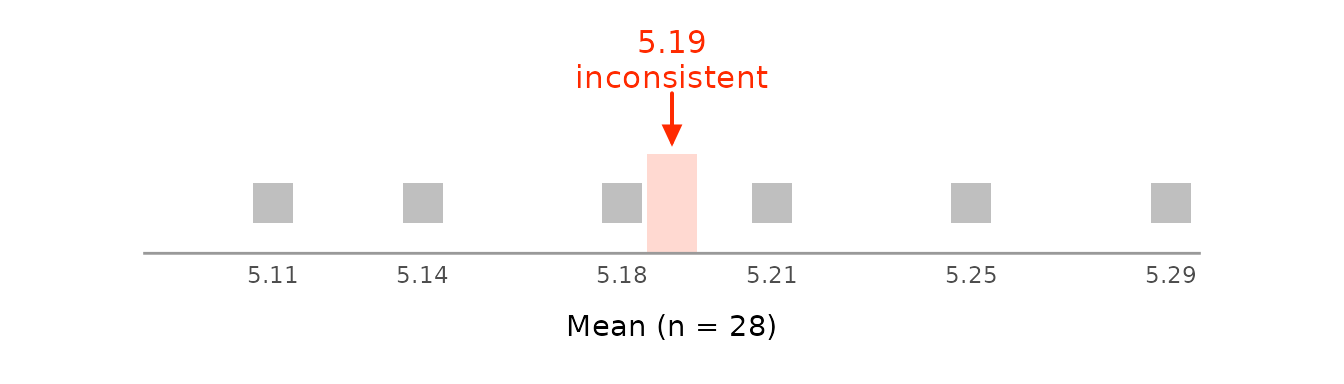

With n = 26, the same mean is consistent:

grim_plot_line(x = 5.19, n = 26, digits_x = 2, items_averaged = 1, data_type = "integer")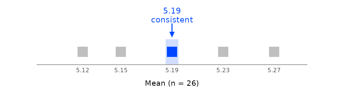

By default, the plot shows the reported value and the nearest achievable one. zoom = "medium" widens it to the nearest achievable value on either side, and zoom = "wide" to a whole unit.

grimmer_plot_line() is the same figure over standard deviations; see vignette("grimmer-in-depth").

The grid behind grim_plot_grid()

grim_grid() returns the grid behind the raster of grim_plot_grid() as a tibble, with GRIM’s result for every cell. It is useful for studying GRIM itself, e.g., the share of means it rules out at each sample size:

grim_grid(digits_x = 2, data_type = "integer") |>
  dplyr::summarise(share_inconsistent = mean(!consistency), .by = n)
#> # A tibble: 100 × 2
#>        n share_inconsistent
#>    <int>              <dbl>
#>  1     1             1     
#>  2     2             0.9899
#>  3     3             0.9798
#>  4     4             0.9697
#>  5     5             0.9596
#>  6     6             0.9495
#>  7     7             0.9394
#>  8     8             0.8889
#>  9     9             0.9192
#> 10    10             0.9091
#> # ℹ 90 more rows

Values around the reported ones: grim_map_seq()

An inconsistency may come from a small error in reporting or computing. grim_map_seq() varies x and n a few steps up and down, one at a time, and tests each resulting value set:

out_seq1 <- grim_map_seq(pigs1, digits_x = 2, items_averaged = 1, data_type = "integer")
out_seq1
#> # A tibble: 160 × 10
#> # GRIM: default settings
#>        x     n items_averaged data_type digits_x consistency exp_incon diff_var
#>    <dbl> <int>          <int> <chr>        <int> <lgl>           <dbl>    <int>
#>  1  4.69    25              1 integer          2 FALSE            0.75       -5
#>  2  4.7     25              1 integer          2 FALSE            0.75       -4
#>  3  4.71    25              1 integer          2 FALSE            0.75       -3
#>  4  4.72    25              1 integer          2 TRUE             0.75       -2
#>  5  4.73    25              1 integer          2 FALSE            0.75       -1
#>  6  4.75    25              1 integer          2 FALSE            0.75        1
#>  7  4.76    25              1 integer          2 TRUE             0.75        2
#>  8  4.77    25              1 integer          2 FALSE            0.75        3
#>  9  4.78    25              1 integer          2 FALSE            0.75        4
#> 10  4.79    25              1 integer          2 FALSE            0.75        5
#> # ℹ 150 more rows
#> # ℹ 2 more variables: case <int>, var <chr>

By default, only inconsistent value sets are dispersed. case is the row in the input data, var the variable that was varied, and diff_var the number of steps from the reported value.

Summaries with audit()

audit() summarizes this output per case:

audit(out_seq1)
#> # A tibble: 8 × 14
#>       x     n items_averaged data_type consistency hits_total hits_x hits_n
#>   <dbl> <int>          <int> <chr>     <lgl>            <int>  <int>  <int>
#> 1  4.74    25              1 integer   FALSE                4      2      2
#> 2  5.23    29              1 integer   FALSE                6      3      3
#> 3  2.57    24              1 integer   FALSE                6      3      3
#> 4  6.77    27              1 integer   FALSE                7      3      4
#> 5  7.01    29              1 integer   FALSE                3      3      0
#> 6  3.14    27              1 integer   FALSE                6      3      3
#> 7  6.89    31              1 integer   FALSE                8      4      4
#> 8  0.24    28              1 integer   FALSE                6      3      3
#> # ℹ 6 more variables: diff_x <int>, diff_x_up <int>, diff_x_down <int>,
#> #   diff_n <int>, diff_n_up <int>, diff_n_down <int>

• x and n are the reported values, and consistency their test result.
• hits_total, hits_x, hits_n: the number of consistent value sets found, in total and by varying each variable.
• diff_x: the distance from x to the nearest consistent value, in dispersion steps. diff_x_up and diff_x_down are the distances to the nearest consistent value above and below. The diff_n* columns are the same for n.

The default dispersion is 1:5, for five steps up and down. With more steps, more hits are typically found:

out_seq2 <- grim_map_seq(
  pigs1,
  digits_x = 2,
  items_averaged = 1,
  data_type = "integer",
  dispersion = 1:10
)
audit(out_seq2)
#> # A tibble: 8 × 14
#>       x     n items_averaged data_type consistency hits_total hits_x hits_n
#>   <dbl> <int>          <int> <chr>     <lgl>            <int>  <int>  <int>
#> 1  4.74    25              1 integer   FALSE               12      6      6
#> 2  5.23    29              1 integer   FALSE               12      6      6
#> 3  2.57    24              1 integer   FALSE               11      6      5
#> 4  6.77    27              1 integer   FALSE               11      6      5
#> 5  7.01    29              1 integer   FALSE                6      6      0
#> 6  3.14    27              1 integer   FALSE               13      6      7
#> 7  6.89    31              1 integer   FALSE               12      6      6
#> 8  0.24    28              1 integer   FALSE               13      6      7
#> # ℹ 6 more variables: diff_x <int>, diff_x_up <int>, diff_x_down <int>,
#> #   diff_n <int>, diff_n_up <int>, diff_n_down <int>

explain_print() explains the rows of this output like those of grim_map(), so you can see why a nearby value passes:

out_seq1 |>
  dplyr::filter(consistency) |>
  explain_print(1)
#> GRIM test: x = 4.72, n = 25, items_averaged = 1, data_type = "integer"
#> 
#> The mean was reported as 4.72, with 2 decimal places. Before rounding (assuming
#> either rounding up from 5 or down from 5), it could have been anything from
#> 4.715 to 4.725.
#> 
#> The mean of 25 integers is their sum divided by 25. So the sum must be from
#> 4.715 * 25 = 117.875 to 4.725 * 25 = 118.125.
#> 
#> A sum of integers is itself an integer, and 118 is in this range:
#> 118 / 25 = 4.72, which rounds to 4.72.
#> 
#> ==> Consistent

Plotting dispersed values

grim_plot_grid() accepts this output. Each reported value set appears as a cross: the horizontal arm consists of the dispersed n values, the vertical arm of the dispersed x values:

grim_plot_grid(out_seq1)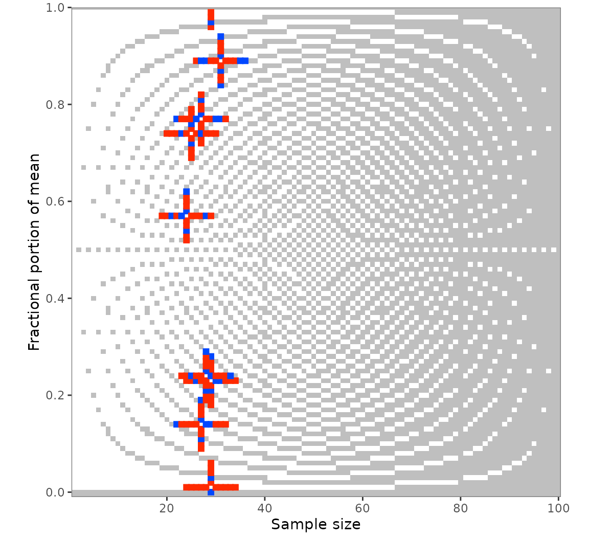

Restrict the dispersion to one variable with var:

out_seq1_only_n <- grim_map_seq(
  pigs1,
  digits_x = 2,
  items_averaged = 1,
  data_type = "integer",
  var = "n"
)
grim_plot_grid(out_seq1_only_n)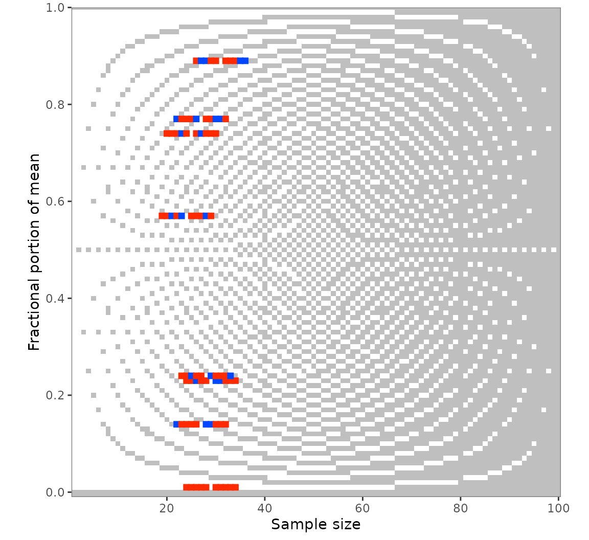

Unknown group sizes: grim_map_total_n()

Some studies report group means but only the total sample size. GRIM can then test hypothetical group sizes: start from an even split, move one participant at a time from one group to the other, and record which splits make both means consistent. grim_map_total_n() does this, following an analysis by Bauer and Francis (2021).

The study they examined reported means of 4.71 and 5.3 for a total of 40 participants. With 20 in each group, only 5.3 is consistent. Bauer and Francis moved to 19/21, 18/22, and 17/23, and found that both means are consistent at 17/23 with 4.71 in the smaller group.

df <- tibble::tibble(x1 = 4.71, x2 = 5.3, n = 40)

df_tested <- grim_map_total_n(df, digits_x = c(2, 1), items_averaged = 1, data_type = "integer")
df_tested
#> # A tibble: 22 × 11
#> # GRIM: default settings
#>        x     n n_change items_averaged data_type digits_x consistency
#>    <dbl> <int>    <int>          <int> <chr>        <int> <lgl>      
#>  1  4.71    20        0              1 integer          2 FALSE      
#>  2  5.3     20        0              1 integer          1 TRUE       
#>  3  4.71    19       -1              1 integer          2 FALSE      
#>  4  5.3     21        1              1 integer          1 TRUE       
#>  5  4.71    18       -2              1 integer          2 FALSE      
#>  6  5.3     22        2              1 integer          1 TRUE       
#>  7  4.71    17       -3              1 integer          2 TRUE       
#>  8  5.3     23        3              1 integer          1 TRUE       
#>  9  4.71    16       -4              1 integer          2 FALSE      
#> 10  5.3     24        4              1 integer          1 TRUE       
#> # ℹ 12 more rows
#> # ℹ 4 more variables: both_consistent <lgl>, exp_incon <dbl>, case <int>,
#> #   dir <fct>

audit(df_tested)
#> # A tibble: 1 × 8
#>      x1    x2     n hits_total hits_forth hits_back scenarios_total hit_rate
#>   <dbl> <dbl> <int>      <int>      <int>     <int>           <int>    <dbl>
#> 1  4.71   5.3    40          3          1         2              11   0.2727

Each row is one mean with one hypothetical group size. n_change is how far that size is from half the total, both_consistent says whether both means of the split are consistent, and dir says which way the means were paired with the groups (see below). A hit is a split in which both means are consistent with their hypothetical group sizes. The default dispersion = 0:5 goes five steps away from the even split.

The two means were reported with different numbers of decimal places, so digits_x has one value per group. Testing 5.3 as if it were 5.30 would be stricter than the test Bauer and Francis conducted.

grim_map_total_n() tests both ways of pairing the means with the group sizes. Bauer and Francis only paired 4.71 with the smaller group; the reverse pairing yields two more hits, at 19/21 and 16/24. In the summary, hits_forth counts the hits from the first pairing, hits_back those from the reverse one, and hits_total their sum. scenarios_total is the number of scenarios tested, each a split with one pairing of the means, and hit_rate the share of them that are hits. The even split is the same scenario under both pairings, so it counts once: six splits make 11 scenarios here.

GRIM statistics

The probability of GRIM inconsistency

The exp_incon column of grim_map() is, for the simplest rounding methods,

$$P = \max\left(0, \frac{10^D - NL}{10^D}\right)$$

where $D$ is the number of decimal places, $N$ the sample size, and $L$ the number of items. This is the probability that a mean with $D$ decimal places but random decimal digits is GRIM-inconsistent with $N$ and $L$. If it is 0, GRIM cannot detect any inconsistency.

The formula is exact for rounding methods in which exactly one range of unrounded values, one rounding step wide, is rounded to each reported value, such as "up". The default, "up_or_down", accepts a mean exactly halfway between two reportable values in both directions, so the formula overstates the probability whenever $NL < 10^D$ and $NL / \gcd(NL, 10^D)$ is even: at $N = 40$ with two decimal places, the probability is $0.4$, not $0.6$. Under "ceiling_or_floor", the range is two steps wide. grim_exp_incon() and grim_total() therefore take rounding and threshold arguments and count exactly the values that grim() would reject. grim_map() passes its own rounding on.

grim_exp_incon(x = 1.40, n = 72, digits_x = 2, items_averaged = 1, data_type = "integer")
#> [1] 0.24

grim_exp_incon(x = 5.93, n = 80, digits_x = 2, items_averaged = 3, data_type = "integer")
#> [1] 0

grim_exp_incon(
  x = 84.27,
  n = 40,
  digits_x = 2,
  items_averaged = 1,
  data_type = "integer",
  x_meaning = "percentage"
)
#> [1] 0.996

grim_total() returns a count instead of a proportion: the number of the $10^D$ possible fractional parts that are inconsistent:

grim_total(x = 1.40, n = 72, digits_x = 2, items_averaged = 1, data_type = "integer")
#> [1] 24

The formula is implicit in Brown and Heathers (2017), who note (p. 367) that with two decimal places and $N < 100$, a random mean is consistent in about $N$% of cases.

A study’s rate of inconsistency

Correctly reported means are always consistent, so a study’s rate of inconsistent value sets should be zero. If the decimal digits of its means were random, that rate would be expected to be the mean of the exp_incon column. grim_binomial() tests whether the rate of consistent value sets is above what random digits would produce. It uses the Poisson binomial distribution, since the probability differs between value sets, and returns the observed consistency rate with a Clopper-Pearson confidence interval:

pigs1 |>
  grim_map(digits_x = 2, items_averaged = 1, data_type = "integer") |>
  grim_binomial()
#> # A tibble: 1 × 9
#>   estimate statistic p.value parameter conf.low conf.high conf.level method     
#>      <dbl>     <int>   <dbl>     <int>    <dbl>     <dbl>      <dbl> <chr>      
#> 1   0.3333         4  0.4531        12   0.1229         1       0.95 Poisson bi…
#> # ℹ 1 more variable: alternative <chr>

grim_binomial_power() computes the power of this test for a given number of value sets, so you can judge whether the test is informative before interpreting its p-value:

grim_binomial_power(p0 = 0.5, p1 = 0.9, k = 10)
#> [1] 0.7360989

Both functions are experimental. grim_plot_rates() shows the same comparison for several studies. Each point is a study, placed at its observed rate of inconsistency against the rate that random means would show; the point area is the number of testable value sets. A study on the dotted line at zero is as expected, and one on the dashed diagonal is as inconsistent as random digits:

# fmt: skip
codes <- c(
  "B", "B", "C", "C", "A", "C",
  "A", "D", "A", "A", "A", "A"
)

pigs1 |>
  grim_map(digits_x = 2, items_averaged = 1, data_type = "integer") |>
  dplyr::mutate(study = codes) |>
  grim_plot_rates(study)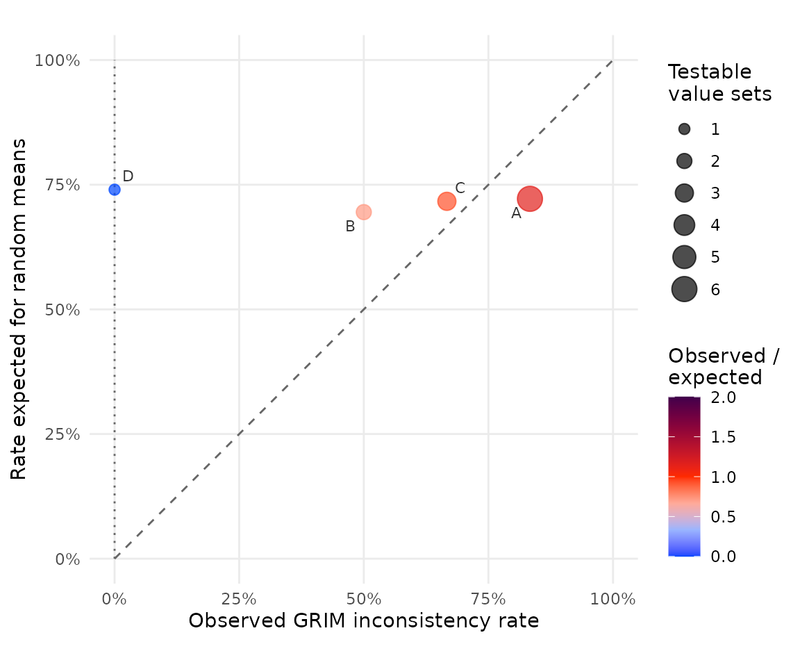

Granularity

The granularity of a scale is the smallest difference between two means it can produce, $G = 1 / (NL)$. grim_granularity() computes it:

grim_granularity(n = 80, items_averaged = 5)
#> [1] 0.0025

References

Bauer, Patricia J., and Gregory Francis. 2021. “Expression of Concern: Is It Light or Dark? Recalling Moral Behavior Changes Perception of Brightness.” Psychological Science 32 (12): 2042–43.

Brown, Nicholas J. L., and James A. J. Heathers. 2017. “The GRIM Test: A Simple Technique Detects Numerous Anomalies in the Reporting of Results in Psychology.” Social Psychological and Personality Science 8 (4): 363–69.