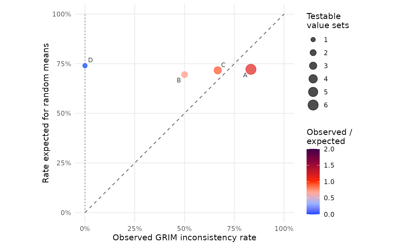

grim_plot_rates() plots one point per study: its observed rate
of GRIM-inconsistent value sets against the rate that means with random
decimal digits would show at the same sample sizes and numbers of decimal
places. This helps spot both problematic studies and problems in GRIM
usage. See Details.
Correctly reported means are always consistent, so a study off the dotted line at zero has a problem, either in the study or in the GRIM analysis. The dashed diagonal marks studies where GRIM inconsistencies are as frequent as expected if the means' digits were random.
Arguments
- data
Data frame returned by
grim_map().- study
<
tidy-select> Column ofdatathat identifies the study of each value set.
Details
The expected rate of a study is the mean of the exp_incon
column, from grim_exp_incon(). Value sets whose exp_incon is zero
or missing are left out because GRIM cannot test them; if none remain,
that is an error. Value sets without a study are left out with a warning.
Point area is the number of GRIM-testable value sets. Color shows the ratio of the observed rate to the expected one: 0 means no inconsistencies, 1 as many as random means. Studies under the diagonal are above 1, in darker colors.
Nothing should push a study's rate above chance, so a large point clearly below the diagonal points to an error in the GRIM analysis. A small point can land there by chance.
See also
grim_binomial() for a test of the same comparison.