Visualize the means that GRIM admits

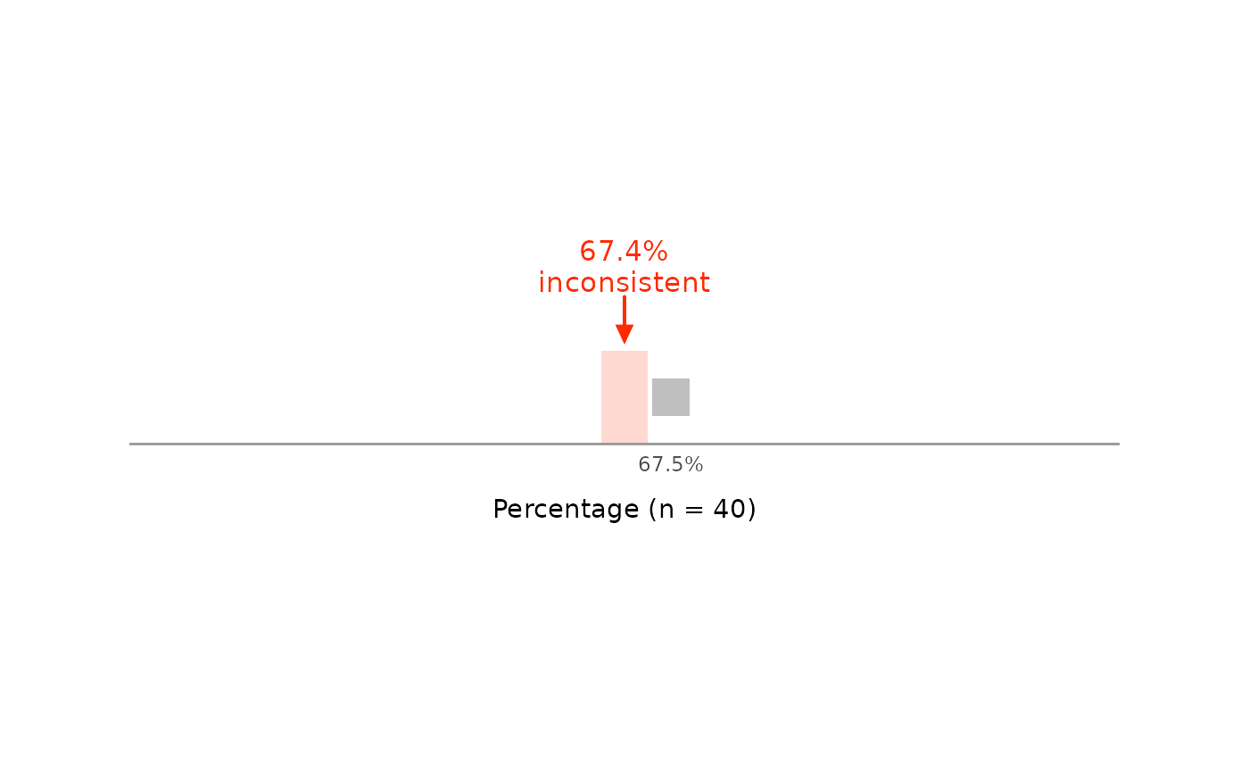
grim_plot_line() draws the GRIM test for a single value set as a row of squares. Of all means (or percentages) that could have been reported with digits_x decimal places, each square is one that a sample of size n can have; the others are left out. The reported value is marked above the row and labeled as consistent or inconsistent.

grim_plot_grid() shows many results at once; this function explains one. grim_values() lists the unrounded means behind a reported one.

Usage

grim_plot_line(
  x,
  n,
  digits_x,
  items_averaged,
  data_type,
  x_meaning = c("mean", "percentage"),
  rounding = "up_or_down",
  threshold = 5,
  symmetric = FALSE,
  zoom = c("close", "medium", "wide"),
  color_con = "#0047ff",
  color_incon = "#ff2a00",
  color_attainable = "grey75"
)

Arguments

x, n, digits_x, items_averaged, x_meaning, rounding, threshold, symmetric

The same as in grim(), but x, n, digits_x, and items_averaged must have length 1.

data_type

String. "integer" if the values are whole numbers, as in grim(). There is no default, so that every call states this assumption. "continuous" and NA are errors: if the data may be continuous, there are no values to draw.

zoom

String. How much of the row to show: "close" (the default), "medium", or "wide"; see Details.

color_con, color_incon

Strings. Color of the marker, the strip behind the squares, and the square at the reported value if it is consistent. color_con applies if the value is consistent, color_incon if not. Defaults are "#0047ff" and "#ff2a00".

color_attainable

String. Color of the squares for attainable values that were not reported, like the consistent cells of grim_plot_grid()'s raster. Default is "grey75".

Value

A ggplot object.

Details

With zoom = "close", the row shows 10 values on either side of x, so that the marker and the strip behind it stand out. If x is inconsistent, it widens until the nearest attainable value is in view, but no farther than the row with zoom = "wide" is wide. It does not widen further for the nearest one on the other side: attainable percentages in particular can be dozens of values apart, so the squares and the strip would shrink to specks.

With zoom = "medium", the row widens until the nearest attainable value other than x is in view on either side, whether x is consistent or not, which shows how far apart the attainable values are. Again, it widens no farther than the row with zoom = "wide". Both settings test at most 20,000 values, and warn if they stop short of an attainable value for that reason.

Each attainable value is labeled below its square unless the squares are too close together for that, as they mostly are with zoom = "wide". Then the axis has the usual breaks, and if x is inconsistent, the nearest attainable values are labeled above the row.

With zoom = "wide", the row runs from the whole number at or below x to the next one up. With items_averaged = 1, about n of the values in this unit are attainable, or all if n exceeds 10 ^ digits_x. With x_meaning = "percentage", the unit is that of the proportion GRIM tests, so the row runs from 0% to 100%, and about n + 1 values are attainable, or all if n exceeds 10 ^ (digits_x + 2). Squares too narrow to be seen as such are drawn as ticks of the same height.

The strip behind the squares is the range of unrounded means that would have been reported as x, from roundwork::unround(). The value is consistent exactly if a square stands within the strip. Under methods such as "trunc" or "ceiling", one edge of the strip is not part of it, so a square on that edge does not count.

See also

grimmer_plot_line() for the same figure over standard deviations.

Examples

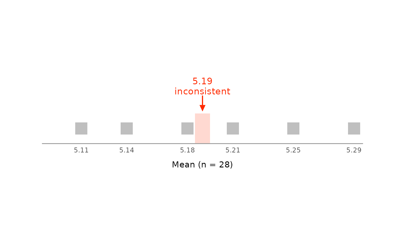
# A mean of 5.19 is not consistent with a sample size of 28:
# no square stands where the marker points.
grim_plot_line(x = 5.19, n = 28, digits_x = 2, items_averaged = 1, data_type = "integer")


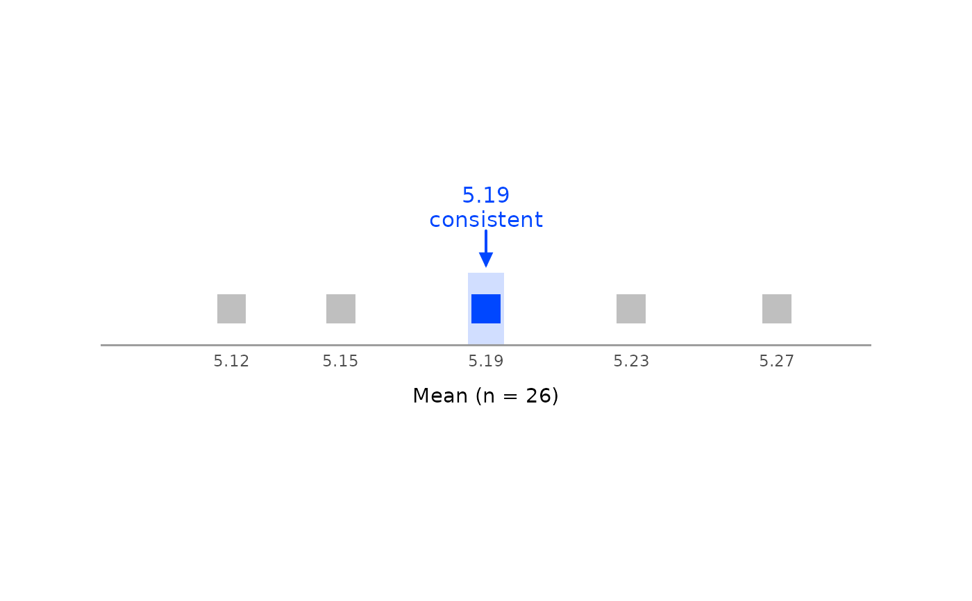
# With `n = 26`, it is:
grim_plot_line(x = 5.19, n = 26, digits_x = 2, items_averaged = 1, data_type = "integer")


# The same for a percentage:
grim_plot_line(
  x = 67.4,
  n = 40,
  digits_x = 1,
  items_averaged = 1,
  data_type = "integer",
  x_meaning = "percentage"
)