
This vignette builds on vignette("grimmer"), which
covers the basics of GRIMMER testing with grimmer() and
grimmer_map(). Here are SDs computed by other conventions,
bounded scales, the means and SDs behind a test result, plots, and the
values around the reported ones with grimmer_map_seq() and
grimmer_map_total_n(). The last few work like their GRIM
counterparts in vignette("grim-in-depth").
Sample or population SD
GRIMMER takes the SD to be a sample SD, which divides by
.
A population SD, as from NumPy’s np.std() or Excel’s
STDEV.P, divides by
.
At small
,
such an SD often fails the test as a sample SD. The values 2, 4, 4, 5,
and 7 have a mean of 4.4 and a population SD of 1.62:
grimmer(
  x = 4.4,
  sd = 1.62,
  n = 5,
  digits_x = 1,
  digits_sd = 2,
  items_averaged = 1,
  data_type = "integer"
)
#> [1] FALSE
grimmer(
  x = 4.4,
  sd = 1.62,
  n = 5,
  digits_x = 1,
  digits_sd = 2,
  items_averaged = 1,
  data_type = "integer",
  sd_meaning = "sd_pop"
)
#> [1] TRUE
sd_meaning = "sd_sample_or_pop" accepts a value set that
is consistent under either convention, and the reason
column of grimmer_map() says which one. It accepts more SDs
than either convention alone, and a study has most likely computed all
its SDs the same way, so testing under "sd_sample" and
"sd_pop" separately tells you more.
sd_meaning = "se" tests whether a standard error was
reported as an SD. This test is weak: the SE was rounded, so the SD may
lie in a range sqrt(n) times as wide. Beyond very small
samples, nearly every value set passes, so a consistent result under
"se" is no evidence that an SE was reported.
Bounded scales
GRIMMER does not use the bounds of a scale. For data on a bounded
scale, such as a five-point Likert scale, see the strait package, whose
brimmest() decides exactly whether a mean and SD are
possible within the bounds.
Achievable means and SDs
grimmer_values() returns every pair of a mean and an SD
that a sample of n integers can have and that would be
reported as x and sd, with the sum and sum of
squares behind each. It is the counterpart of
grim_values(), and like it, it returns one row per
achievable pair, with case for the value set, and none if
the value set is inconsistent:
grimmer_values(
  x = 5.3,
  sd = 0.7,
  n = 30,
  digits_x = 1,
  digits_sd = 1,
  items_averaged = 1,
  data_type = "integer"
)
#> # A tibble: 7 × 7
#>    case     x     sd     n items_averaged   sum sum_squares
#>   <int> <dbl>  <dbl> <int>          <int> <dbl>       <dbl>
#> 1     1 5.267 0.6915    30              1   158         846
#> 2     1 5.267 0.7397    30              1   158         848
#> 3     1 5.3   0.6513    30              1   159         855
#> 4     1 5.3   0.7022    30              1   159         857
#> 5     1 5.3   0.7497    30              1   159         859
#> 6     1 5.333 0.6609    30              1   160         866
#> 7     1 5.333 0.7112    30              1   160         868
grimmer_values(
  x = 5.23,
  sd = 2.55,
  n = 35,
  digits_x = 2,
  digits_sd = 2,
  items_averaged = 1,
  data_type = "integer"
)
#> # A tibble: 0 × 7
#> # ℹ 7 variables: case <int>, x <dbl>, sd <dbl>, n <int>, items_averaged <int>,
#> #   sum <dbl>, sum_squares <dbl>
With the sum and sum of squares of each group, a statistic that
combines several groups, such as a t-value, can be recomputed
for every possible sample and compared with the reported one.
sd_meaning = "sd_sample_or_pop" is not allowed here: the
same sum of squares gives a different SD under each premise, so call the
function once for each.
grimmer_closest() returns the one pair whose SD is
closest to the reported one, like grim_closest() for means.
For an inconsistent value set, this shows how far off the SD is:
grimmer_closest(
  x = 5.23,
  sd = 2.55,
  n = 35,
  digits_x = 2,
  digits_sd = 2,
  items_averaged = 1,
  data_type = "integer"
)
#> # A tibble: 1 × 7
#>    case     x    sd     n items_averaged   sum sum_squares
#>   <int> <dbl> <dbl> <int>          <int> <dbl>       <dbl>
#> 1     1 5.229 2.545    35              1   183        1177
A single value set: grimmer_plot_line()
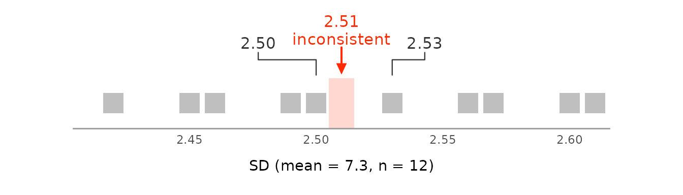
grimmer_plot_line() draws the test for a single value
set, like grim_plot_line() does for means; it helps to
explain a result. It shows the SDs that could have been reported around
the reported one and marks those that a sample with the given mean and
size can have:
grimmer_plot_line(
  x = 7.3,
  sd = 2.51,
  n = 12,
  digits_x = 1,
  digits_sd = 2,
  items_averaged = 1,
  data_type = "integer"
)
Many value sets: grim_plot_grid()
grim_plot_grid() accepts grimmer_map()
output. The raster shows the GRIM part of the test, and each value set
is colored by its GRIMMER result. A red value set on a grey cell passed
GRIM but failed GRIMMER, and a message counts these:
pigs5 |>
  grimmer_map(digits_x = 2, digits_sd = 2, items_averaged = 1, data_type = "integer") |>
  grim_plot_grid()
#> → Also visualizing 1 GRIMMER inconsistency.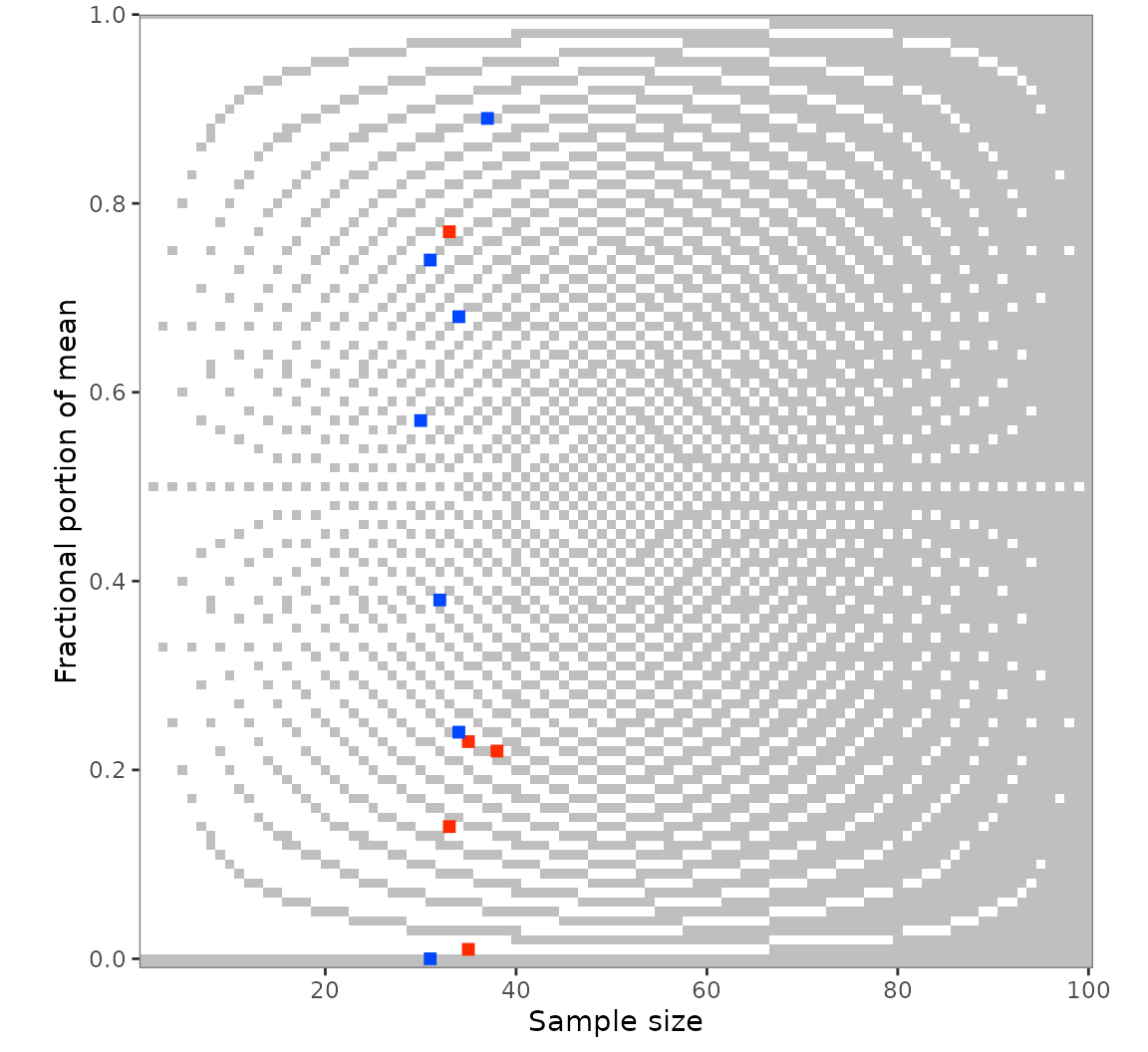
Values around the reported ones: grimmer_map_seq()
grimmer_map_seq() varies x,
sd, and n around the reported values, by
default only for inconsistent value sets:
out_seq1 <- grimmer_map_seq(
  pigs5,
  digits_x = 2,
  digits_sd = 2,
  items_averaged = 1,
  data_type = "integer"
)
out_seq1
#> # A tibble: 150 × 12
#> # GRIMMER: default settings
#>        x    sd     n items_averaged data_type digits_x digits_sd consistency
#>    <dbl> <dbl> <int>          <int> <chr>        <int>     <int> <lgl>
#>  1  7.17   5.3    38              1 integer          2         2 FALSE
#>  2  7.18   5.3    38              1 integer          2         2 TRUE
#>  3  7.19   5.3    38              1 integer          2         2 FALSE
#>  4  7.2    5.3    38              1 integer          2         2 FALSE
#>  5  7.21   5.3    38              1 integer          2         2 TRUE
#>  6  7.23   5.3    38              1 integer          2         2 FALSE
#>  7  7.24   5.3    38              1 integer          2         2 TRUE
#>  8  7.25   5.3    38              1 integer          2         2 FALSE
#>  9  7.26   5.3    38              1 integer          2         2 TRUE
#> 10  7.27   5.3    38              1 integer          2         2 FALSE
#> # ℹ 140 more rows
#> # ℹ 4 more variables: reason <chr>, diff_var <int>, case <int>, var <chr>

audit(out_seq1)
#> # A tibble: 5 × 19
#>       x    sd     n items_averaged data_type consistency hits_total hits_x
#>   <dbl> <dbl> <int>          <int> <chr>     <lgl>            <int>  <int>
#> 1  7.22  5.3     38              1 integer   FALSE                8      4
#> 2  5.23  2.55    35              1 integer   FALSE               15      2
#> 3  6.77  2.18    33              1 integer   FALSE                5      3
#> 4  7.01  6.68    35              1 integer   FALSE                4      4
#> 5  3.14  5.32    33              1 integer   FALSE                9      4
#> # ℹ 11 more variables: hits_sd <int>, hits_n <int>, diff_x <int>,
#> #   diff_x_up <int>, diff_x_down <int>, diff_sd <int>, diff_sd_up <int>,
#> #   diff_sd_down <int>, diff_n <int>, diff_n_up <int>, diff_n_down <int>
The summary is the same as for GRIM, with hits_sd and
the diff_sd* columns added. More steps typically find more
hits:
out_seq2 <- grimmer_map_seq(
  pigs5,
  digits_x = 2,
  digits_sd = 2,
  items_averaged = 1,
  data_type = "integer",
  dispersion = 1:10
)
audit(out_seq2)
#> # A tibble: 5 × 19
#>       x    sd     n items_averaged data_type consistency hits_total hits_x
#>   <dbl> <dbl> <int>          <int> <chr>     <lgl>            <int>  <int>
#> 1  7.22  5.3     38              1 integer   FALSE               15      8
#> 2  5.23  2.55    35              1 integer   FALSE               30      6
#> 3  6.77  2.18    33              1 integer   FALSE               10      4
#> 4  7.01  6.68    35              1 integer   FALSE                8      8
#> 5  3.14  5.32    33              1 integer   FALSE               14      7
#> # ℹ 11 more variables: hits_sd <int>, hits_n <int>, diff_x <int>,
#> #   diff_x_up <int>, diff_x_down <int>, diff_sd <int>, diff_sd_up <int>,
#> #   diff_sd_down <int>, diff_n <int>, diff_n_up <int>, diff_n_down <int>
grim_plot_grid() accepts this output as well, and
var restricts the dispersion to one variable:
out_seq1_only_n <- grimmer_map_seq(
  pigs5,
  digits_x = 2,
  digits_sd = 2,
  items_averaged = 1,
  data_type = "integer",
  var = "n"
)
grim_plot_grid(out_seq1_only_n)
#> → Also visualizing 2 GRIMMER inconsistencies.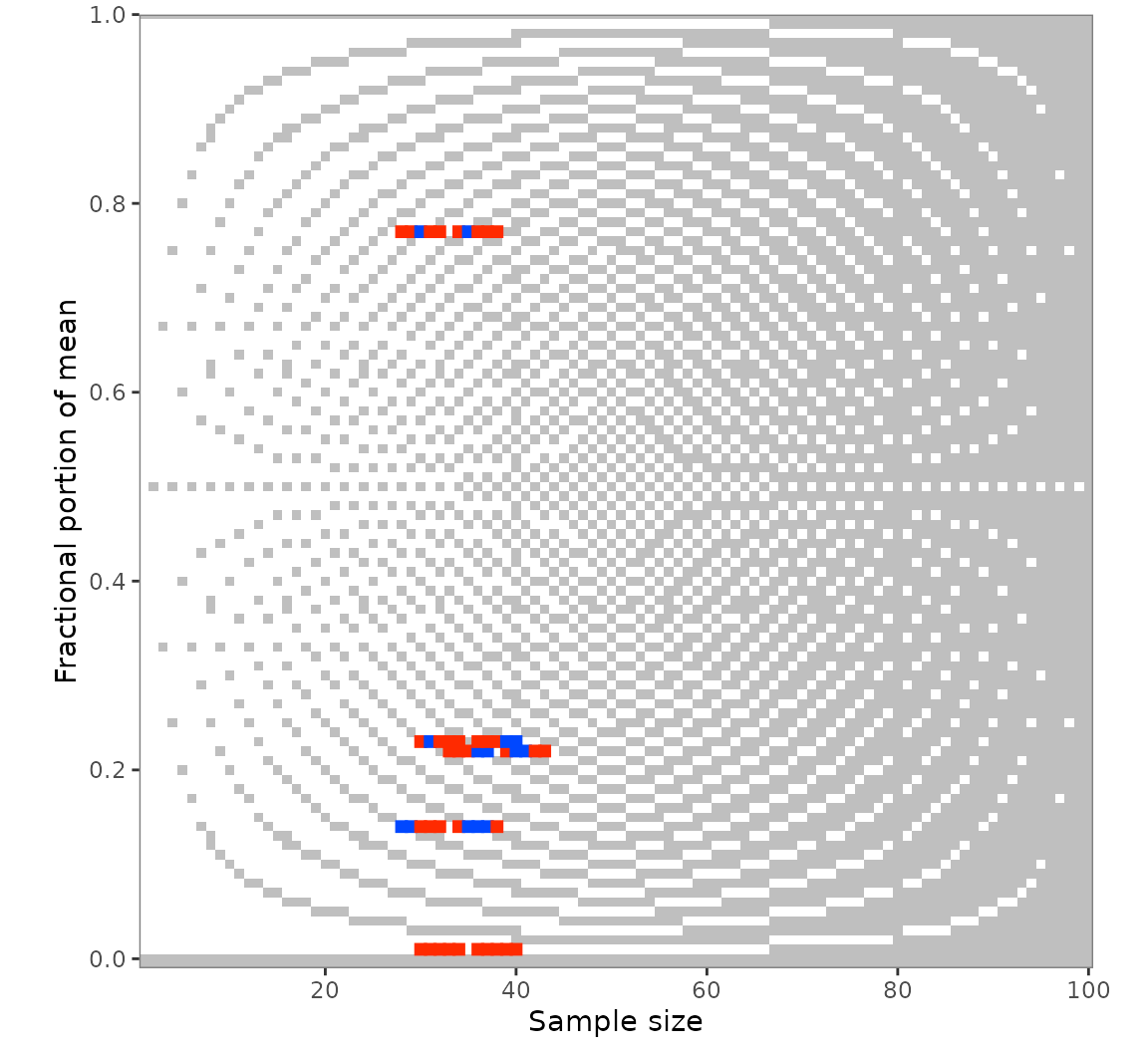
Unknown group sizes: grimmer_map_total_n()
If only the total sample size of two groups is known,
grimmer_map_total_n() tests hypothetical splits of it, as
grim_map_total_n() does; see
vignette("grim-in-depth") for a case study.
flying_pigs4 <- tibble::tribble(
  ~x1  , ~x2  , ~sd1 , ~sd2 , ~n ,
  3.91 , 3.89 , 1.38 , 1.47 , 70 ,
  3.77 , 4.37 , 1.74 , 1.44 , 65
)

out_total_n <- grimmer_map_total_n(
  flying_pigs4,
  digits_x = 2,
  digits_sd = 2,
  items_averaged = 1,
  data_type = "integer"
)
out_total_n
#> # A tibble: 46 × 13
#> # GRIMMER: default settings
#>        x    sd     n n_change items_averaged data_type digits_x digits_sd
#>    <dbl> <dbl> <int>    <int>          <int> <chr>        <int>     <int>
#>  1  3.91  1.38    35        0              1 integer          2         2
#>  2  3.89  1.47    35        0              1 integer          2         2
#>  3  3.91  1.38    34       -1              1 integer          2         2
#>  4  3.89  1.47    36        1              1 integer          2         2
#>  5  3.91  1.38    33       -2              1 integer          2         2
#>  6  3.89  1.47    37        2              1 integer          2         2
#>  7  3.91  1.38    32       -3              1 integer          2         2
#>  8  3.89  1.47    38        3              1 integer          2         2
#>  9  3.91  1.38    31       -4              1 integer          2         2
#> 10  3.89  1.47    39        4              1 integer          2         2
#> # ℹ 36 more rows
#> # ℹ 5 more variables: consistency <lgl>, both_consistent <lgl>, reason <chr>,
#> #   case <int>, dir <fct>

audit(out_total_n)
#> # A tibble: 2 × 10
#>      x1    x2   sd1   sd2     n hits_total hits_forth hits_back scenarios_total
#>   <dbl> <dbl> <dbl> <dbl> <int>      <int>      <int>     <int>           <int>
#> 1  3.91  3.89  1.38  1.47    70          4          4         0              11
#> 2  3.77  4.37  1.74  1.44    65          1          1         0              12
#> # ℹ 1 more variable: hit_rate <dbl>