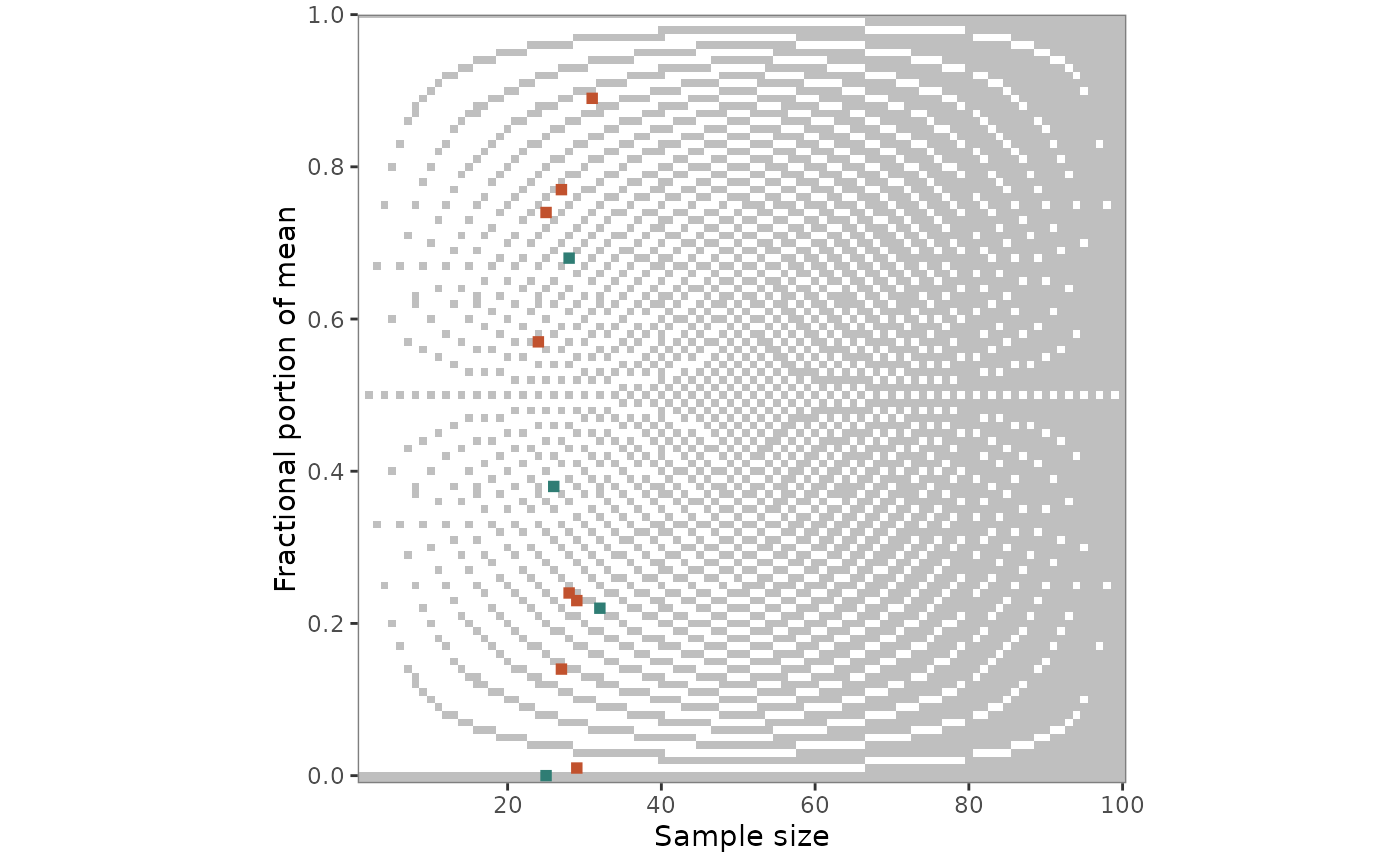
Visualize GRIM test results — grim_plot

grim_plot_grid() plots the output of grim_map() or grimmer_map(). Each value set is placed by n * items_averaged (the sample size for single items) and the fractional part of its mean, in blue if consistent and red if not, on a background raster that shows which combinations are GRIM-consistent at all.

Usage

grim_plot_grid(
  data = NULL,
  show_data = TRUE,
  show_raster = TRUE,
  show_gradient = TRUE,
  split_by_digits = FALSE,
  n = NULL,
  digits_x = NULL,
  rounding = "up_or_down",
  threshold = 5,
  tile_size = 1.5,
  color_raster = "grey75"
)

Arguments

data: Data frame returned by grim_map() or grimmer_map(), or by their *_seq() and *_total_n() variants.
show_data: Logical. If FALSE, only the raster is drawn. Default is TRUE.
show_raster: Logical. Should the raster be drawn? Default is TRUE.
show_gradient: Logical. With three or more decimal places, should a gradient be drawn? Default is TRUE.
split_by_digits: Logical. If TRUE, return a named list with one plot per number of decimal places instead of erroring when they differ. Cannot be combined with digits_x. Default is FALSE.
n: Integer. Maximal value on the x-axis. Default is NULL, in which case the axis spans the raster and the data.
digits_x: Integer. Number of decimal places for the raster. Default is NULL, in which case it is read from the digits_x column that every mapper adds, or, if that was removed, inferred from x, which loses trailing zeros. With show_data = FALSE, NULL means 2. For percentages, give the number of decimal places as reported; 2 are added.
rounding, threshold: The same as in grim(), for the raster. Only used if show_data is FALSE: otherwise, the raster follows the settings of the mapper call, and giving others is an error. Defaults are "up_or_down" and 5.
tile_size: Numeric. Size of the tiles for value sets. Default is 1.5.
color_raster: String. Color of the consistent cells of the raster, and of the consistent end of the gradient that replaces it with three or more decimal places. Default is "grey75".

Value

A ggplot object. With split_by_digits = TRUE, a named list of ggplot objects, one per distinct non-zero number of decimal places (e.g., list(digits_1 = ..., digits_2 = ...)), returned invisibly after each plot is printed.

Background raster

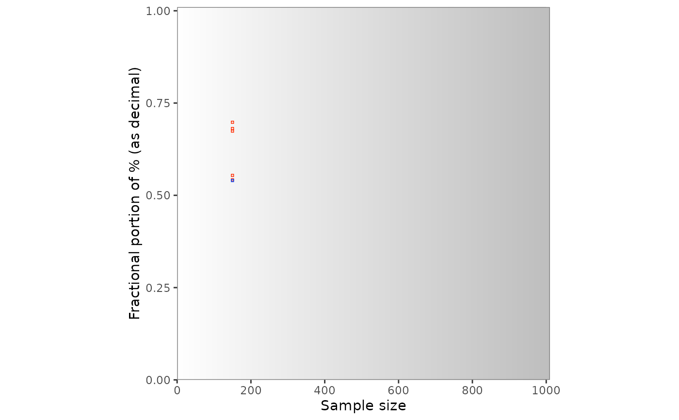
For one or two decimal places, the raster shows every combination of sample size and fractional part that is GRIM-consistent in grey and every inconsistent one in white. It depends on the number of decimal places, which is read from the digits_x column of data, and on the rounding method, which is read from the grim_map() call. The white tiles are the cells of grim_grid() whose consistency is FALSE. With three or more decimal places, they would be too small, so a gradient shows the probability of inconsistency instead.

A raster only applies to one number of decimal places, so grim_plot_grid() errors if digits_x varies across rows. Use split_by_digits = TRUE to get one plot per number of decimal places instead, or digits_x to choose one.

With x_meaning = "percentage" in the grim_map() call, percentages are plotted as the proportions they were tested as, with two more decimal places.

Set show_data = FALSE to plot the raster alone, controlled by digits_x, rounding, threshold, and n.

Under the default rounding = "up_or_down", fewer values are inconsistent at sample sizes 40 and 80 than at their neighbors with two decimal places (4 and 8 with one), and none at 80 (or 8), because many achievable means there are ties, which the default accepts in both directions.

Negative means

The y-axis is the fractional part of the absolute value of x, so a mean of -2.51 is drawn at 0.51. GRIM's granularity is symmetric around zero, so this is the value set's place on the grid. A one-directional rounding method treats the absolute value of a negative number the other way: "ceiling" like "floor", and "up" like "down" (unless symmetric = TRUE). If all means are negative, the raster is the one for this mirrored method, so that it agrees with the tiles. With positive and negative means under such a method, no single raster does; it is then the one for positive means, with a warning. The tile's color comes from the consistency column and is unaffected.

References

Brown, N. J. L., & Heathers, J. A. J. (2017). The GRIM Test: A Simple Technique Detects Numerous Anomalies in the Reporting of Results in Psychology. Social Psychological and Personality Science, 8(4), 363–369. https://journals.sagepub.com/doi/10.1177/1948550616673876

Examples

# `grim_plot_grid()` reads the number of decimal places
# from the `digits_x` column:
pigs1 |>
  grim_map(digits_x = 2, items_averaged = 1, data_type = "integer") |>
  grim_plot_grid()


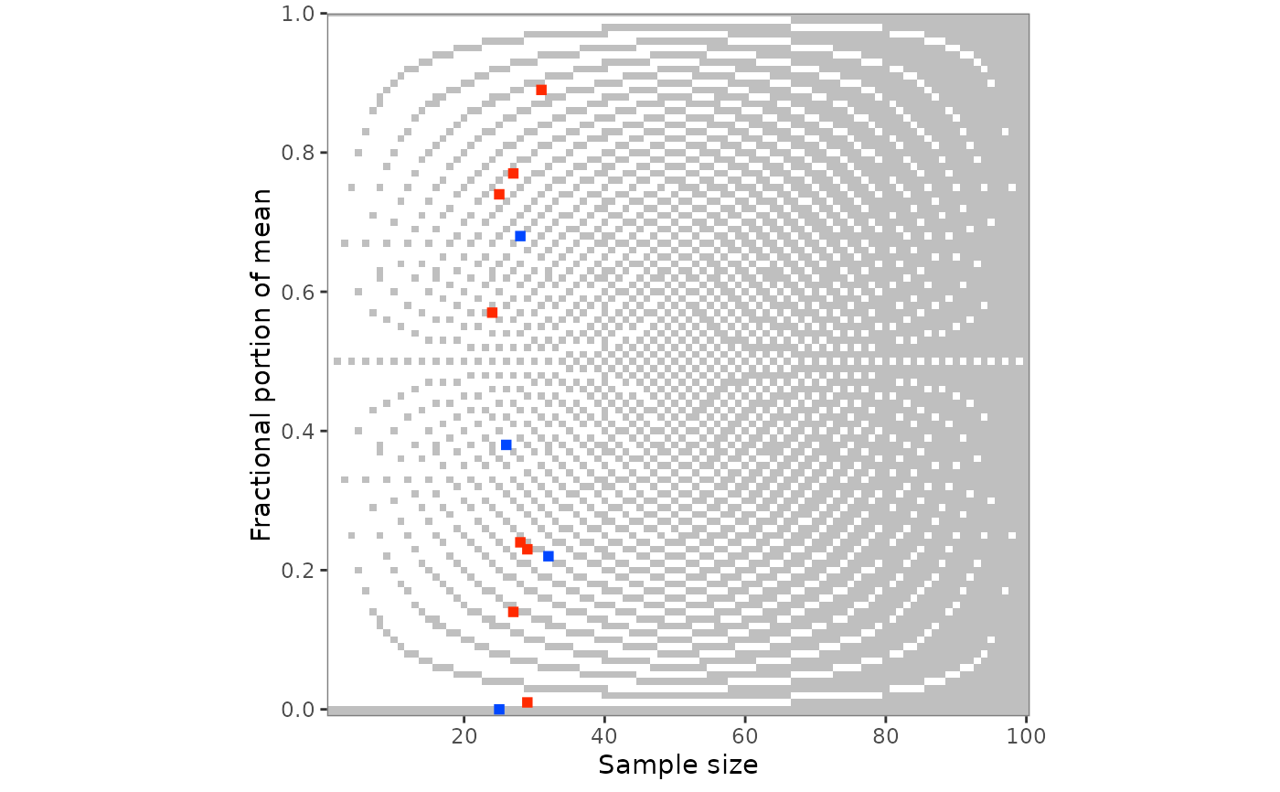# The raster follows the rounding method of the `grim_map()` call:
pigs1 |>
  grim_map(
    digits_x = 2,
    items_averaged = 1,
    data_type = "integer",
    rounding = "ceiling"
  ) |>
  grim_plot_grid()


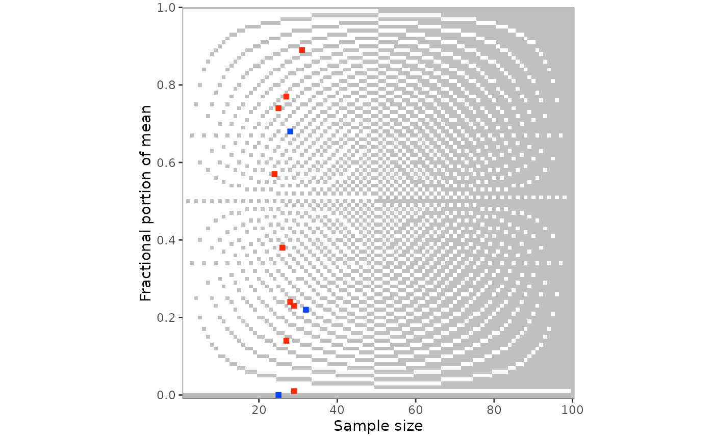# Percentages are plotted as proportions:
pigs2 |>
  grim_map(
    digits_x = 1,
    items_averaged = 1,
    data_type = "integer",
    x_meaning = "percentage"
  ) |>
  grim_plot_grid()


# Other colors for the value sets:
pigs1 |>
  grim_map(digits_x = 2, items_averaged = 1, data_type = "integer") |>
  grim_plot_grid() +
  ggplot2::scale_colour_manual(
    values = c("TRUE" = "#2f7d74", "FALSE" = "#c1522e"),
    aesthetics = c("colour", "fill"),
    guide = "none"
  )
#> Scale for colour is already present.
#> Adding another scale for colour, which will replace the existing scale.