Generate CLOSURE samples — closure

Call closure_generate() to run the CLOSURE algorithm on a given set of summary statistics.

This can take seconds, minutes, or longer, depending on the input. Wide variance and large n often lead to many samples, i.e., long runtimes. These effects interact dynamically. For example, with large n, even very small increases in sd can greatly increase runtime and number of values found.

If the inputs are inconsistent, there is no solution. The function will then return empty results and throw a warning.

Usage

closure_generate(
  mean,
  sd,
  n,
  scale_min,
  scale_max,
  rounding = "up_or_down",
  threshold = 5,
  warn_if_empty = TRUE,
  ask_to_proceed = TRUE,
  rounding_error_mean = NULL,
  rounding_error_sd = NULL
)

Arguments

mean: String (length 1). Reported mean.
sd: String (length 1). Reported sample standard deviation.
n: Numeric (length 1). Reported sample size.
scale_min, scale_max: Numeric (length 1 each). Minimal and maximal possible values of the measurement scale. For example, with a 1-7 Likert scale, use scale_min = 1 and scale_max = 7. Prefer the empirical min and max if available: they constrain the possible values further.
rounding: String (length 1). Rounding method assumed to have created mean and sd. See Rounding options, but also the Rounding limitations section below. Default is "up_or_down" which, e.g., unrounds 0.12 to 0.115 as a lower bound and 0.125 as an upper bound.
threshold: Numeric (length 1). Number from which to round up or down, if rounding is any of "up_or_down", "up", and "down". Default is 5.
warn_if_empty: Logical (length 1). Should a warning be shown if no samples are found? Default is TRUE.
ask_to_proceed: Logical (length 1). If the runtime is predicted to be very long, should the function prompt you to proceed or abort in an interactive setting? Default is TRUE.
rounding_error_mean, rounding_error_sd: Numeric (length 1 each). Option to manually set the rounding error around mean and sd. This is meant for development and might be removed in the future, so most users can ignore it.

Value

Named list of four tibbles (data frames):

inputs: Arguments to this function.
metrics:
- samples_initial: integer. The basis for computing CLOSURE results, based on scale range only. See closure_count_initial().
- samples_all: integer. Number of all samples. Equal to the number of rows in results.
- values_all: integer. Number of all individual values found. Equal to n * samples_all.
- horns: double. Measure of dispersion for bounded scales; see horns().
- horns_uniform: double. Value horns would have if the reconstructed sample was uniformly distributed.
frequency:
- value: integer. Scale values derived from scale_min and scale_max.
- f_average: Count of scale values in the mean results sample.
- f_absolute: integer. Count of individual scale values found in the results samples.
- f_relative: double. Values' share of total values found.
results:
- id: integer. Runs from 1 to samples_all.
- sample: list of integer vectors. Each of these vectors has length n. It is a sample (or distribution) of individual scale values found by CLOSURE.

Rounding limitations

The rounding and threshold arguments are not fully implemented. For example, CLOSURE currently treats all rounding bounds as inclusive, even if the rounding specification would imply otherwise.

Many specifications of the two arguments will not make any difference, and those that do will most likely lead to empty results.

Examples

# High spread often leads to many samples --
# here, 3682.
data_high <- closure_generate(
  mean = "3.5",
  sd = "1.7",
  n = 70,
  scale_min = 1,
  scale_max = 5
)

data_high
#> $inputs
#> # A tibble: 1 × 7
#>   mean  sd        n scale_min scale_max rounding   threshold
#>   <chr> <chr> <dbl>     <dbl>     <dbl> <chr>          <dbl>
#> 1 3.5   1.7      70         1         5 up_or_down         5
#> 
#> $metrics
#> # A tibble: 1 × 5
#>   samples_initial samples_all values_all horns horns_uniform
#>             <int>       <int>      <int> <dbl>         <dbl>
#> 1              15        2492     174440 0.708           0.5
#> 
#> $frequency
#> # A tibble: 5 × 4
#>   value f_average f_absolute f_relative
#>   <int>     <dbl>      <int>      <dbl>
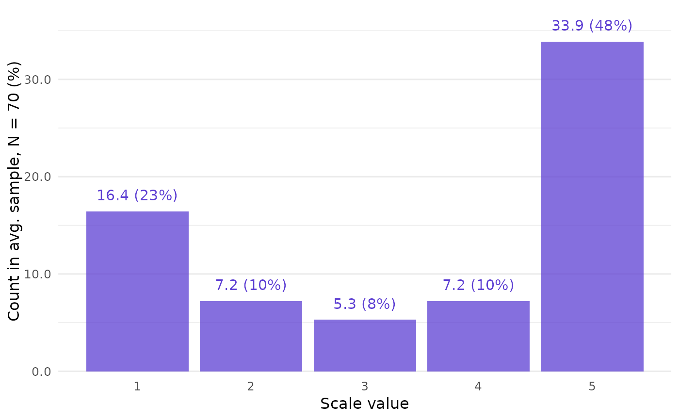
#> 1     1     16.4       40982     0.235 
#> 2     2      7.19      17922     0.103 
#> 3     3      5.29      13172     0.0755
#> 4     4      7.19      17916     0.103 
#> 5     5     33.9       84448     0.484 
#> 
#> $results
#> # A tibble: 2,492 × 2
#>       id sample    
#>    <int> <list>    
#>  1     1 <int [70]>
#>  2     2 <int [70]>
#>  3     3 <int [70]>
#>  4     4 <int [70]>
#>  5     5 <int [70]>
#>  6     6 <int [70]>
#>  7     7 <int [70]>
#>  8     8 <int [70]>
#>  9     9 <int [70]>
#> 10    10 <int [70]>
#> # ℹ 2,482 more rows
#> 

# Get a clear picture of the distribution
# by following up with `closure_plot_bar()`:
closure_plot_bar(data_high)


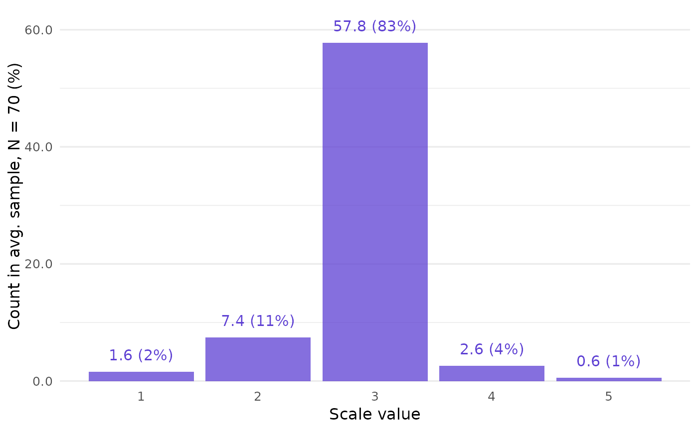
# Low spread, only 3 samples, and not all
# scale values are possible.
data_low <- closure_generate(
  mean = "2.9",
  sd = "0.5",
  n = 70,
  scale_min = 1,
  scale_max = 5
)

data_low
#> $inputs
#> # A tibble: 1 × 7
#>   mean  sd        n scale_min scale_max rounding   threshold
#>   <chr> <chr> <dbl>     <dbl>     <dbl> <chr>          <dbl>
#> 1 2.9   0.5      70         1         5 up_or_down         5
#> 
#> $metrics
#> # A tibble: 1 × 5
#>   samples_initial samples_all values_all  horns horns_uniform
#>             <int>       <int>      <int>  <dbl>         <dbl>
#> 1              15         219      15330 0.0643           0.5
#> 
#> $frequency
#> # A tibble: 5 × 4
#>   value f_average f_absolute f_relative
#>   <int>     <dbl>      <int>      <dbl>
#> 1     1     1.59         349    0.0228 
#> 2     2     7.42        1626    0.106  
#> 3     3    57.8        12659    0.826  
#> 4     4     2.61         572    0.0373 
#> 5     5     0.566        124    0.00809
#> 
#> $results
#> # A tibble: 219 × 2
#>       id sample    
#>    <int> <list>    
#>  1     1 <int [70]>
#>  2     2 <int [70]>
#>  3     3 <int [70]>
#>  4     4 <int [70]>
#>  5     5 <int [70]>
#>  6     6 <int [70]>
#>  7     7 <int [70]>
#>  8     8 <int [70]>
#>  9     9 <int [70]>
#> 10    10 <int [70]>
#> # ℹ 209 more rows
#> 

# This can also be shown by `closure_plot_bar()`:
closure_plot_bar(data_low)