Visualize rates of ignored NAs

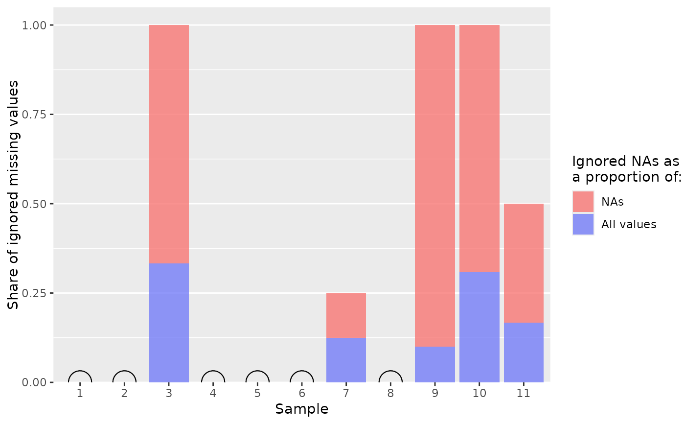
median_plot_col() visualizes the results of median_table(). It shows the rates of missing values that had to be ignored to estimate the median of the remaining values.

Usage

median_plot_col(
  data,
  bar_alpha = 0.8,
  bar_color_na = "#F77774",
  bar_color_all = "#747DF7",
  ring_color = "black",
  ring_size = 8,
  show_ring = TRUE,
  show_legend = TRUE
)

Arguments

data

Data frame returned by median_table().

bar_alpha

Numeric. Opacity of the bars. Default is 0.4.

bar_color_na, bar_color_all

Strings. Colors of the bars representing the number of missing values that had to be ignored as a share of all missing values (_na) or of the entire sample (_all).

ring_color

String. Color of any "ring of certainty" half circle. Default is "black".

ring_size

Numeric. Size of any "ring of certainty" half circle. Default is 8.

show_ring

Logical. Should samples with a known median be marked by a "ring of certainty" half circle? Default is TRUE.

show_legend

Logical. Should a legend be displayed? Default is TRUE. Note: there is no legend if there are no bars.

Value

A ggplot object.

Visual guide (default)

• Red bars show the share of missing values that had to be ignored as a share of all missing values.

• Blue bars show the same but as a share of all values, missing or not. They cover part of the blue bars; both types of bars start at zero.

• The y-axis is fixed between 0 and 1 for a consistent display of proportions.

• Samples without any bar do not require ignoring any NAs, so the median is known. They are also marked by a "ring of certainty", which is just a half circle here.

See also

• median_plot_errorbar() for an alternative visualization.

• median_table() for the basis of these plots.

Examples

# Example data:
data <- median_table(
  list(
    c(0, 1, 1, 1, NA),
    c(1, 1, NA),
    c(1, 2, NA),
    c(0, 0, NA, 0, 0),
    c(1, 1, 1, 1, NA, NA),
    c(1, 1, 1, 1, NA, NA, NA),
    c(1, 1, 1, 1, NA, NA, NA, NA),
    iris$Sepal.Length,
    c(5.6, 5.7, 5.9, 6, 6.1, 6.3, 6.4, 6.6, 6.7, NA),
    c(6.1, 6.3, 5.9, 6, 6.1, 6.3, 6.4, 6.6, 6.7, NA, NA, NA, NA),
    c(7, 7, 7, 8, NA, NA)
  )
)

data
#> # A tibble: 11 × 10
#>    term  estimate certainty lower upper na_ignored na_total rate_ignored_na
#>    <chr>    <dbl> <lgl>     <dbl> <dbl>      <int>    <int>           <dbl>
#>  1 ""         1   TRUE       1      1            0        1            0   
#>  2 ""         1   TRUE       1      1            0        1            0   
#>  3 ""         1.5 FALSE      1      2            1        1            1   
#>  4 ""         0   TRUE       0      0            0        1            0   
#>  5 ""         1   TRUE       1      1            0        2            0   
#>  6 ""         1   TRUE       1      1            0        3            0   
#>  7 ""         1   FALSE     NA     NA            1        4            0.25
#>  8 ""         5.8 TRUE       5.8    5.8          0        0            0   
#>  9 ""         6.1 FALSE      6.05   6.2          1        1            1   
#> 10 ""         6.3 FALSE      6.1    6.4          4        4            1   
#> 11 ""         7   FALSE      7      7.5          1        2            0.5 
#> # ℹ 2 more variables: sum_total <int>, rate_ignored_sum <dbl>

# See visual guide above
median_plot_col(data)